


Using a Convolutional Neural Network to Play Conway's Game of Life with Keras
The goal of this post is to train a neural network to play Conway’s Game of Life without explicitly teaching it the rules of the game.
Speaking of which, if you’re not familiar with Conway’s Game of Life, the rules are as follows:
The universe of the Game of Life is an infinite, two-dimensional orthogonal grid of square cells, each of which is in one of two possible states, alive or dead, (or populated and unpopulated, respectively). Every cell interacts with its eight neighbours, which are the cells that are horizontally, vertically, or diagonally adjacent. At each step in time, the following transitions occur:
- Any live cell with fewer than two live neighbors dies, as if by underpopulation.
- Any live cell with two or three live neighbors lives on to the next generation.
- Any live cell with more than three live neighbors dies, as if by overpopulation.
- Any dead cell with exactly three live neighbors becomes a live cell, as if by reproduction.
The initial pattern constitutes the seed of the system. The first generation is created by applying the above rules simultaneously to every cell in the seed; births and deaths occur simultaneously, and the discrete moment at which this happens is sometimes called a tick. Each generation is a pure function of the preceding one. The rules continue to be applied repeatedly to create further generations.
Why do this? Mostly for fun, and to learn a little bit about convolutional neural networks. It’s probably overkill for Conway’s Game, but it’s still pretty interesting to see how it performs.
Without further ado, let’s jump into it.
Game Logic
The first thing to do is define a function that takes a game board as input and returns the next state. Luckily there are plenty of implementations available online, such as the following from https://jakevdp.github.io/blog/2013/08/07/conways-game-of-life/. Basically, it takes a game board matrix as input where 0 represents a dead cell and 1 represents a living cell, and returns a matrix of the same size but containing the state of each cell on the next iteration of the game.
import numpy as np

def life_step(X):
    live_neighbors = sum(np.roll(np.roll(X, i, 0), j, 1)
                     for i in (-1, 0, 1) for j in (-1, 0, 1)
                     if (i != 0 or j != 0))
    return (live_neighbors == 3) | (X & (live_neighbors == 2)).astype(int)
Generate Game Boards
With the game logic in place, the next thing we’ll want is some way to randomly generate game boards (frames) and a way to visualize them. generate_frames creates num_frames random game boards with a particular shape and a predefined probability of each cell being ‘alive’, and render_frames draws image representations of two game boards side-by-side for comparison, where living cells are white and dead cells are black:
import matplotlib.pyplot as plt

def generate_frames(num_frames, board_shape=(100,100), prob_alive=0.15):
    return np.array([
        np.random.choice([False, True], size=board_shape, p=[1-prob_alive, prob_alive])
        for _ in range(num_frames)
    ]).astype(int)

def render_frames(frame1, frame2):
    plt.subplot(1, 2, 1)
    plt.imshow(frame1.flatten().reshape(board_shape), cmap='gray')

    plt.subplot(1, 2, 2)
    plt.imshow(frame2.flatten().reshape(board_shape), cmap='gray')
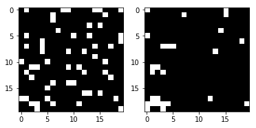
Let’s see what these frames look like:
board_shape = (20, 20)
board_size = board_shape[0] * board_shape[1]
probability_alive = 0.15

frames = generate_frames(10, board_shape=board_shape, prob_alive=probability_alive)
print(frames.shape) # (num_frames, board_w, board_h)
(10, 20, 20)
print(frames[0])
[[0, 0, 0, 1, 0, 0, 1, 1, 0, 0, 1, 0, 0, 0, 1, 0, 0, 0, 1, 0],
 [0, 0, 0, 0, 1, 0, 0, 0, 0, 0, 0, 1, 0, 0, 0, 0, 0, 0, 1, 1],
 [0, 0, 0, 0, 0, 0, 0, 0, 0, 0, 0, 0, 1, 0, 1, 0, 1, 0, 0, 0],
 [0, 0, 0, 0, 0, 0, 0, 0, 0, 0, 0, 0, 0, 0, 1, 0, 1, 0, 0, 0],
 [0, 0, 0, 0, 0, 0, 0, 0, 0, 0, 0, 0, 0, 0, 1, 0, 0, 0, 0, 0],
 [0, 1, 0, 0, 0, 0, 0, 1, 0, 1, 0, 0, 0, 0, 0, 0, 0, 0, 0, 0],
 [0, 0, 0, 0, 0, 0, 0, 0, 0, 0, 0, 0, 0, 0, 0, 0, 0, 0, 0, 0],
 [0, 0, 0, 0, 0, 0, 0, 0, 0, 0, 0, 0, 0, 0, 0, 0, 0, 0, 0, 0],
 [0, 0, 0, 0, 0, 0, 0, 0, 0, 0, 1, 0, 0, 0, 1, 0, 0, 0, 0, 1],
 [0, 0, 0, 0, 0, 0, 0, 0, 0, 0, 1, 0, 0, 0, 0, 0, 1, 0, 1, 1],
 [1, 0, 0, 0, 1, 0, 1, 0, 0, 0, 1, 0, 0, 0, 0, 0, 0, 0, 0, 0],
 [0, 0, 0, 0, 0, 1, 0, 0, 1, 1, 0, 0, 0, 0, 0, 0, 1, 0, 0, 0],
 [1, 0, 0, 0, 0, 1, 1, 0, 0, 0, 0, 0, 0, 0, 1, 0, 0, 0, 0, 0],
 [0, 0, 0, 0, 0, 0, 0, 1, 0, 0, 1, 0, 0, 0, 0, 1, 1, 0, 0, 0],
 [0, 0, 1, 0, 0, 1, 0, 0, 0, 0, 0, 0, 0, 0, 0, 0, 0, 0, 0, 0],
 [0, 0, 0, 0, 0, 0, 1, 0, 0, 0, 0, 0, 0, 0, 1, 0, 0, 0, 0, 0],
 [0, 0, 0, 0, 0, 0, 1, 0, 0, 0, 0, 1, 1, 1, 1, 0, 0, 0, 0, 0],
 [0, 0, 1, 0, 0, 0, 0, 0, 0, 0, 0, 0, 1, 0, 0, 0, 0, 0, 0, 0],
 [0, 0, 0, 1, 0, 0, 0, 1, 1, 0, 0, 0, 0, 0, 1, 0, 0, 0, 0, 0],
 [0, 0, 1, 0, 0, 0, 0, 0, 0, 0, 0, 0, 0, 0, 1, 0, 1, 0, 1, 0]])
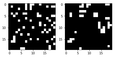
The following takes the integer representation of a game board from above, and renders it as an image. To the right it also renders the next state of the game board using the life_step function:
render_frames(frames[1], life_step(frames[1]))
Construct a Training and Validation Set
Now that we can generate data, we’ll generate training, validation and test sets.
Each element in the y_train/y_val/y_test arrays will represent the next Game of Life board for each board frame in X_train/X_val/X_test.
def reshape_input(X):
    return X.reshape(X.shape[0], X.shape[1], X.shape[2], 1)

def generate_dataset(num_frames, board_shape, prob_alive):
    X = generate_frames(num_frames, board_shape=board_shape, prob_alive=prob_alive)
    X = reshape_input(X)
    y = np.array([
        life_step(frame)
        for frame in X
    ])
    return X, y

train_size = 70000
val_size   = 10000
test_size  = 20000
print("Training Set:")
X_train, y_train = generate_dataset(train_size, board_shape, probability_alive)
print(X_train.shape)
print(y_train.shape)
Training Set:
(70000, 20, 20, 1)
(70000, 20, 20, 1)
print("Validation Set:")
X_val, y_val = generate_dataset(val_size, board_shape, probability_alive)
print(X_val.shape)
print(y_val.shape)
Validation Set:
(10000, 20, 20, 1)
(10000, 20, 20, 1)
print("Test Set:")
X_test, y_test = generate_dataset(test_size, board_shape, probability_alive)
print(X_test.shape)
print(y_test.shape)
Test Set:
(20000, 20, 20, 1)
(20000, 20, 20, 1)
Build a Convolutional Neural Network
Now we can take a first crack at building a Convolutional Neural Network using Keras. The key here is the kernel_size of (3, 3) and strides of 1. This instructs the CNN to look at a 3x3 matrix of surrounding cells for each 1 cell of the board it looks at, including the current cell itself.
For example, if the following were a game board and we were at the middle cell x, it would look at all the cells marked with an exclamation mark ! and the x cell. It would then move along 1 cell to the right, and do the same, repeating over and over until it’s looked at every cell, and its neighbors, of the entire board.
0 0 0 0 0
0 ! ! ! 0
0 ! x ! 0
0 ! ! ! 0
0 0 0 0 0
The rest of the network is pretty basic, so I won’t go into much detail about it. If you’re curious about anything, I’d recommend checking out the documentation for the class in question.
from keras.models import Sequential
from keras.layers import Dense, Dropout, Activation, Conv2D, MaxPool2D

# CNN Properties
filters = 50
kernel_size = (3, 3) # look at all 8 neighboring cells, plus itself
strides = 1
hidden_dims = 100

model = Sequential()
model.add(Conv2D(
    filters,
    kernel_size,
    padding='same',
    activation='relu',
    strides=strides,
    input_shape=(board_shape[0], board_shape[1], 1)
))
model.add(Dense(hidden_dims))
model.add(Dense(1))
model.add(Activation('sigmoid'))

model.compile(loss='binary_crossentropy', optimizer='adam', metrics=['accuracy'])
Let’s look at the model using the summary function:
model.summary()
_________________________________________________________________
Layer (type)                 Output Shape              Param #
=================================================================
conv2d_9 (Conv2D)            (None, 20, 20, 50)        500
_________________________________________________________________
dense_17 (Dense)             (None, 20, 20, 100)       5100
_________________________________________________________________
dense_18 (Dense)             (None, 20, 20, 1)         101
_________________________________________________________________
activation_9 (Activation)    (None, 20, 20, 1)         0
=================================================================
Total params: 5,701
Trainable params: 5,701
Non-trainable params: 0
_________________________________________________________________
Train and Save the Model
With the CNN defined, let’s train the model and save it to disk:
def train(model, X_train, y_train, X_val, y_val, batch_size=50, epochs=2, filename_suffix=''):
    model.fit(
        X_train, y_train,
        batch_size=batch_size,
        epochs=epochs,
        validation_data=(X_val, y_val)
    )

    with open('cgol_cnn{}.json'.format(filename_suffix), 'w') as file:
        file.write(model.to_json())
    model.save_weights('cgol_cnn{}.h5'.format(filename_suffix))


train(model, X_train, y_train, X_val, y_val, filename_suffix='_basic')
Train on 70000 samples, validate on 10000 samples
Epoch 1/2
70000/70000 [==============================] - 27s 388us/step
    - loss: 0.1324 - acc: 0.9651 - val_loss: 0.0833 - val_acc: 0.9815
Epoch 2/2
70000/70000 [==============================] - 27s 383us/step
    - loss: 0.0819 - acc: 0.9817 - val_loss: 0.0823 - val_acc: 0.9816
This model achieves a little over 98% accuracy on both the training and validation sets, which is pretty good for a first pass. Let’s try to figure out where we’re making mistakes.
Try it Out
Let’s take a look at a prediction for a random game board and see how it does. First, generate a single game board and take a look at the correct subsequent frame:
X, y = generate_dataset(1, board_shape=board_shape, prob_alive=probability_alive)

render_frames(X[0].flatten().reshape(board_shape), y)
Next, let’s perform the prediction and see how many were cells were incorrectly predicted:
pred = model.predict_classes(X)
print(np.count_nonzero(pred.flatten() - y.flatten()), "incorrect cells.")
4 incorrect cells.
Next, let’s compare the correct next frame versus the predicted frame:
render_frames(y, pred.flatten().reshape(board_shape))
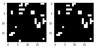
It’s not terrible, but can you see where it failed? It appears to be failing to predict the cells around the edges of the game board. Take a look at the following where non-zero values indicate incorrect predictions:
print(pred.flatten().reshape(board_shape) - y.flatten().reshape(board_shape))
[[ 0  0  0  0  0  0  0 -1  0  0  0  0  0  0  0  0  0 -1 -1  0]
 [ 0  0  0  0  0  0  0  0  0  0  0  0  0  0  0  0  0  0  0  0]
 [ 0  0  0  0  0  0  0  0  0  0  0  0  0  0  0  0  0  0  0  0]
 [ 0  0  0  0  0  0  0  0  0  0  0  0  0  0  0  0  0  0  0  0]
 [ 0  0  0  0  0  0  0  0  0  0  0  0  0  0  0  0  0  0  0  0]
 [ 0  0  0  0  0  0  0  0  0  0  0  0  0  0  0  0  0  0  0  0]
 [ 0  0  0  0  0  0  0  0  0  0  0  0  0  0  0  0  0  0  0  0]
 [ 0  0  0  0  0  0  0  0  0  0  0  0  0  0  0  0  0  0  0  0]
 [ 0  0  0  0  0  0  0  0  0  0  0  0  0  0  0  0  0  0  0  0]
 [ 0  0  0  0  0  0  0  0  0  0  0  0  0  0  0  0  0  0  0  0]
 [ 0  0  0  0  0  0  0  0  0  0  0  0  0  0  0  0  0  0  0  0]
 [ 0  0  0  0  0  0  0  0  0  0  0  0  0  0  0  0  0  0  0  0]
 [ 0  0  0  0  0  0  0  0  0  0  0  0  0  0  0  0  0  0  0  0]
 [ 0  0  0  0  0  0  0  0  0  0  0  0  0  0  0  0  0  0  0  0]
 [ 0  0  0  0  0  0  0  0  0  0  0  0  0  0  0  0  0  0  0  0]
 [ 0  0  0  0  0  0  0  0  0  0  0  0  0  0  0  0  0  0  0  0]
 [ 0  0  0  0  0  0  0  0  0  0  0  0  0  0  0  0  0  0  0  0]
 [ 0  0  0  0  0  0  0  0  0  0  0  0  0  0  0  0  0  0  0  0]
 [ 0  0  0  0  0  0  0  0  0  0  0  0  0  0  0  0  0  0  0  0]
 [ 0  0  0  0  0  0 -1  0  0  0  0  0  0  0  0  0  0  0  0  0]]
As you can see, all of the non-zero values are located on the edges of the game board. Let’s take a look at the full testing set and see if that observation holds true.
View Frequent Errors using Test Set
We’ll write a function that renders a heat map depicting where the model is making errors, and invoke it using the entire testing set:
def view_prediction_errors(model, X, y):
    y_pred = model.predict_classes(X)
    sum_y_pred = np.sum(y_pred, axis=0).flatten().reshape(board_shape)
    sum_y = np.sum(y, axis=0).flatten().reshape(board_shape)

    plt.imshow(sum_y_pred - sum_y, cmap='hot', interpolation='nearest')
    plt.show()

view_prediction_errors(model, X_test, y_test)
All of the errors are around the edges, and the model performs the worst in the corners. This makes sense since the CNN cannot look around the edges, but the Game of Life logic in life_step does. For example, consider the following. Currently, when looking at the edge cell x below, the CNN only sees the x and the ! cells:
0 0 0 0 0
! ! 0 0 0
x ! 0 0 0
! ! 0 0 0
0 0 0 0 0
But what we really want, and what life_step is doing, is to look at the cells on the opposite side as well:
0 0 0 0 0
! ! 0 0 !
x ! 0 0 !
! ! 0 0 !
0 0 0 0 0
The same logic applies to corner cells, like so:
x ! 0 0 !
! ! 0 0 !
0 0 0 0 0
0 0 0 0 0
! 0 0 0 !
To fix this, the padding property of the Conv2D needs to somehow look at the opposite side of the game board. Alternatively, each input board could be pre-processed to pad the edges with the opposite side, and then Conv2D can simply drop the first/last column and row. Since we’re at the mercy of Keras and the padding functionality it provides, which don’t support what we’re looking for, we’ll have to resort to adding our own padding.
Fixing the Edge Issue with Custom Padding
We need to pad each game board with the opposite value to simulate how life_step looks across the game board for edge values. We can use np.pad with mode=’wrap’ to accomplish this. For instance, consider the following array and the padded output below:
x = np.array([
    [1, 2, 3],
    [4, 5, 6],
    [7, 8, 9]
])

print(np.pad(x, (1, 1), mode='wrap'))
[[9, 7, 8, 9, 7],
 [3, 1, 2, 3, 1],
 [6, 4, 5, 6, 4],
 [9, 7, 8, 9, 7],
 [3, 1, 2, 3, 1]]
Notice now how the first column/row and the last column/row are mirrors of the opposite side of the original matrix, and the middle 3x3 matrix is the original value x. For example, cell [1][1] has been replicated on the far side in cell [4][1], and likewise [0][1] contains [3][1]. In every direction, and even in the corners, the array has been wrapped to contain its opposite side, just how we want. This will allow the CNN to consider the wrapped game board and properly handle the edge cases (pun intended).
Now we can write a function to pad all our input matrices:
def pad_input(X):
    return reshape_input(np.array([
        np.pad(x.reshape(board_shape), (1,1), mode='wrap')
        for x in X
    ]))

X_train_padded = pad_input(X_train)
X_val_padded = pad_input(X_val)
X_test_padded = pad_input(X_test)

print(X_train_padded.shape)
print(X_val_padded.shape)
print(X_test_padded.shape)
(70000, 22, 22, 1)
(10000, 22, 22, 1)
(20000, 22, 22, 1)
All the datasets are now padded with their wrapped columns/rows, allowing the CNN to look around the opposite side of the game board just like life_step does. Because of this, each game board is now 22x22 instead of the original 20x20.
Next, the CNN must be reconstructed to drop the padding values using padding=’valid’ (which tells Conv2D to drop the edges, although thats not immediately obvious), and updated to handle the new input_shape. This way when we pass in the padded 22x22 game boards we still get 20x20 game boards as output, since we’ll drop the first and last columns/rows. The rest remains identical:
model_padded = Sequential()
model_padded.add(Conv2D(
    filters,
    kernel_size,
    padding='valid',
    activation='relu',
    strides=strides,
    input_shape=(board_shape[0] + 2, board_shape[1] + 2, 1)
))
model_padded.add(Dense(hidden_dims))
model_padded.add(Dense(1))
model_padded.add(Activation('sigmoid'))

model_padded.compile(loss='binary_crossentropy', optimizer='adam', metrics=['accuracy'])
model_padded.summary()
_________________________________________________________________
Layer (type)                 Output Shape              Param #
=================================================================
conv2d_10 (Conv2D)           (None, 20, 20, 50)        500
_________________________________________________________________
dense_19 (Dense)             (None, 20, 20, 100)       5100
_________________________________________________________________
dense_20 (Dense)             (None, 20, 20, 1)         101
_________________________________________________________________
activation_10 (Activation)   (None, 20, 20, 1)         0
=================================================================
Total params: 5,701
Trainable params: 5,701
Non-trainable params: 0
_________________________________________________________________
Now we can train using the padded inputs:
train(
    model_padded,
    X_train_padded, y_train, X_val_padded, y_val,
    filename_suffix='_padded'
)
Train on 70000 samples, validate on 10000 samples
Epoch 1/2
70000/70000 [==============================] - 27s 389us/step - loss: 0.0604 - acc: 0.9807 - val_loss: 4.5475e-04 - val_acc: 1.0000
Epoch 2/2
70000/70000 [==============================] - 27s 382us/step - loss: 1.7058e-04 - acc: 1.0000 - val_loss: 5.9932e-05 - val_acc: 1.0000
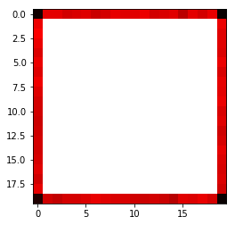
Validation and training accuracy are up to 100% from the roughly 98% we got before adding the padding. Let’s see the test error:
view_prediction_errors(model_padded, X_test_padded, y_test)
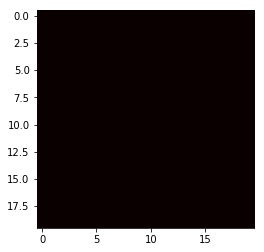
Perfect! The black heat map indicates that there is no variance in the values, meaning we successfully predicted every cell, for every game.
And that’s all there is to it. This was a fun little exercise to play with convolutional neural networks, without requiring a big data set. Feel free to check it out at github.com/KyleBanks/conways-gol-cnn.